Humans like to think and see in straight lines, but the world is curve.
Linear Regression is usually the first data model that everyone learned when they studied data science. The data model is easy to conceptualize, explain and understand by everyone because it is an extension of linear geometry mathematical functions that we all have learnt from school. Input x-values output the y-value and magically predict the next y-value in a straight extrapolating line.
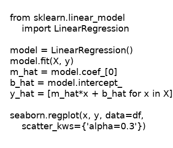
Scikit library contains ready to use powerful data model algorithms. The data models are functions performing gradient descent computations reducing the cost functions. A few lines of code, a magical data model to predict future value is born.
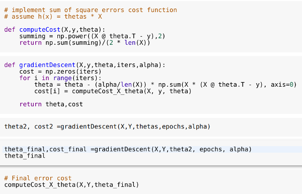
At the core of Regression data model, are the many names of cost function reductions, such as minimum square error, ordinary least square, sum of square error, loss functions, error functions. They are all a flavor of cost optimizer of gradient descent. Gradient descent is the algorithm for finding the minimum cost or error of the functions.
Even though we have the formula to extrapolate y-output label projections into future predictions based on incoming x-values observation data points, the y-output predictions seldom accurately predict future true occurrings most of the time.
In nature of the universe, natural occurrings always fall on shape of a normal bell curve distributions. A single line or sheet of prediction plane slicing through a cloud space of bell curve distribution of possible true y-output predictions, will only be able to predict those true future occurings that exist in the straight path of predictions. This means most of the possible true occurrings that exist above and below the plane of predictions, will not be discovered.
No bulleye prediction, what went wrong
Plotting seaborn regression graph, the thickest bell curve known y-label training output distribution shows the narrowest regression errors as the line of prediction slicing through the denser cloud.
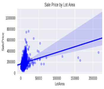
Conversely in region where fewer true known y-label values in existence, the line prediction encounters wider uncertainty as otherwise known as wider regression error. In nature, true occurences that occur above, below or around the y-prediction band projection, will not be accurately predicted or captured.
Looking under the hood of Linear Regression prediction making
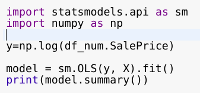
Statsmodel library is a powerful library examining many angle of feature column or dimensional relationships affecting the prediction output. Intuitively, the more dimension or factors affecting the output, the greater the uncertainty and the higher the regression errors will be.
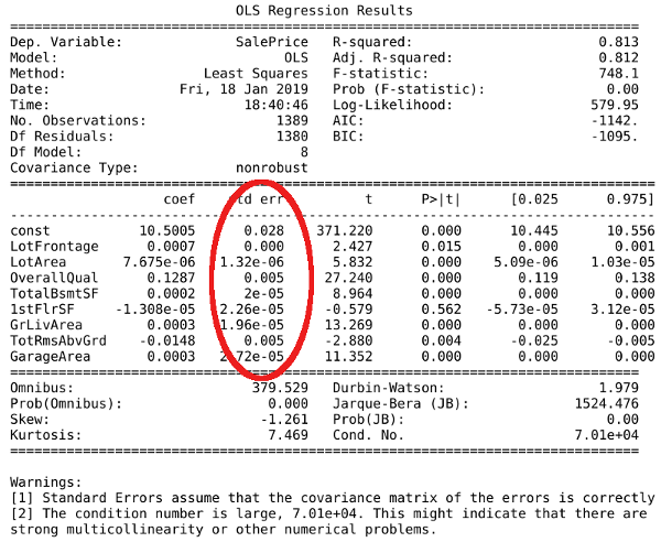
For the purpose of choosing the most direct influential x-dimensional features impacting y-output prediction, we are mostly concerned with the standard error of x-dimensional feature coefficients and multi-collinearity.
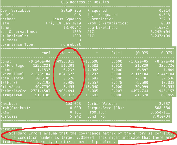

High coefficient standard errors of x-dimensional value features shown above, mean the predicted y-output prediction by Linear Regression model has higher uncertainty as it passes through the cloud of true y-output prediction as shown in the regression graph above.
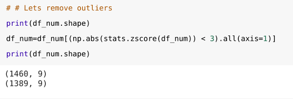
Removing outliers in training dataset, reduce data distraction which help Linear Regression model reduce its coefficient standard errors of x-dimensional features and eventually produce more accurate predictions.
Many ways to reduce regression errors, but most effective way, is to logarithmically transform y-label training output.
Logarithmic transformation has the effect of smoothing out uneven y-label training value into a relatively smooth normal distribution. Thing in nature exists harmoniously in the shape of normal distribution. Hence logarithmically transforming unevenly y-value into denser cloud of smooth normal distribution shape, greatly reduce the uncertainty encountered by the Linear Regression model as it projects its prediction in a straight line through the cloud of true y-values.
By logarithmically transformed y-label training output only, previously high standard errors plaguing coefficient of x-dimensional features, are greatly reduced as shown below.
What caused uncertainty errors or variance in y-prediction
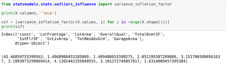
Statsmodel library detects high multi-collinearity in x-dimensional value features if exist.
High multi-collinearity means the data model has x-dimensional features that are highly correlated to each other instead of correlating to y-output prediction. X-dimensional features that behave closely similar to each other, exert higher weighting effect on data model to produce y-output predictions that are biased toward the overly-correlated X-dimensional features. It also makes the data model insensitive to other relevant x-value changes, resulting in higher variance errors.
Removing dimensional features that are closely correlated, will reduce uncertainty errors from y-prediction
To remove multi-collinearity, use Variance-Inflation-Factor functions to identify offending x-dimensional features. X-value features identified by Variance-Inflation-Factor that have value over 10, should be dropped in order to reduce high inter-features correlation.
Dropping all x-value features with high Variance-Inflation-Factor, will systematically tune the Linear Regression data model to best fitting its straight line or plane of predictions through the best possible true y-prediction distributions, with a narrower band of uncertainty errors.
The best Linear Regression still can not accurately predict what it can not see.
Even though uncertainty error or variance can be greatly minimized and eliminated, Linear Regression can only predict accurately whatever possible true occurrings that happen in its path of projections. Possible true future occurrings that happen around that the path of tight band projections, will not be predicted by the Linear Regression model.
Conclusion
If things in nature stay the same over time and the root-cause-effect relationship is one-to-one, then Linear Regression will be the magical future predicting data model. Unfortunately nature operates under the laws of Entropy. What cause and effect in the past, does not guarantee to happen the same in the future as influenced by the laws of Entropy. In nature the root causes to an effect, are many and complex. If a root-cause-effect relationship is such that event X1 causes event X2 and X2 produces Y result outcome, then Linear Regression will fail to recognize this X1=>X2=>Y relationship. Linear Regression can only recognize one-to-one relationship, such as X1=>Y or X2=>Y.
Linear Regression prediction operates under the assumption that the future will occur exactly the same as the past and there are direct one-to-one root-cause-effect relationship. Hence Linear Regression data modeling can only be used in limited situation where the variance of future outcome possibility is toleratedly small and the root cause-effect relationship is direct and one-to-one.
Nevertheless Linear Regression remains popular because it resembles commom human initial overly simplistic reactive thinking, which we all grow accustomed to.